
At what point does the cost of increasing the training dataset size out way any benefit to a model’s predictive performance?
This article aims to provide a heuristic understanding of the relationship between accuracy and training data so that together we can answer that very question.
Training most ML models requires a lot of data (particularly Artificial Neural Networks). In supervised learning cases, a data scientist will need to meticulously label that data.
More training data means the ML model will generalise better to data it has never seen before. Likewise, when the amount of training data is small the model does not generalise well, this is usually because the model is overfitting. In a sense, we are just creating a system that memorises every training input.
Unfortunately, training data is hard to find, often limited by budgetary or time restrictions. In other cases, training data is simply not prevalent enough. Hence, it is important then to analyse the costs and benefits in finding new data.
Set-up
We will be investigating the effect that increasing the training dataset size has on the prediction accuracy of three ML models with varying complexity:
- A custom shallow Artificial Neural Network (ANN)
- A Convolution Neural Network (CNN) built with TensorFlow
- A Support Vector Machine (SVM) Algorithm
To keep the experiment consistent, we will train each model to classify handwritten digits with the MNIST dataset (the “hello world” of computer vision).
As the training size increases the number of epochs, learning rate, and regularisation parameter will be adjusted accordingly to control the impact they might have on the accuracy of the model (and make sure training completes in a reasonable amount of time).
All the code used to generate any artefacts can be found in this GitHub repository.
Investigation
Accuracy vs Training Sample Size
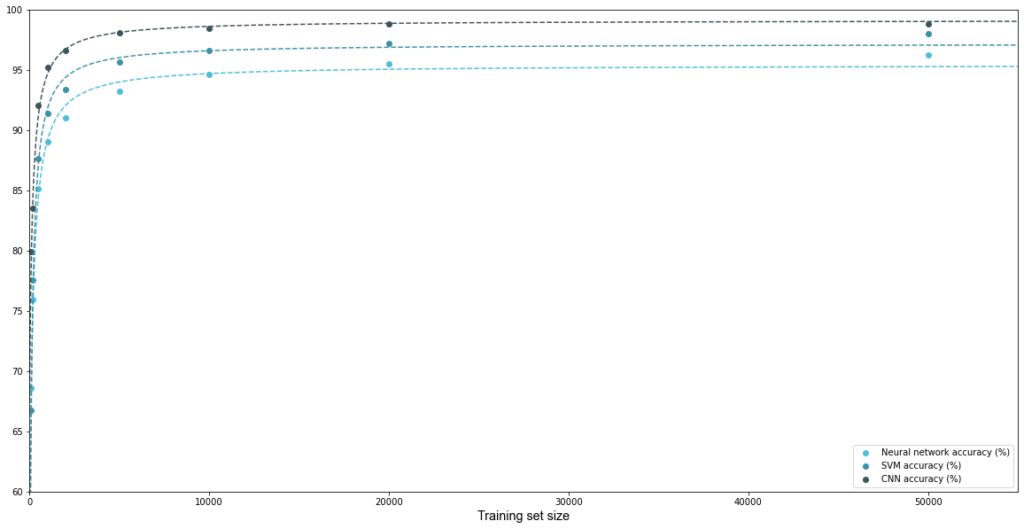
Figure 1 below shows a slowdown of accuracy improvement as we increase the training sample size beyond 500 training samples. The slowdown is characterised by a sharp increase in prediction accuracy followed by a rapid flattening of the curve.

Notably, this behaviour is present in all three models, hence we can deduce that it is not inherent to a particular ML architecture.
As a first pass, we can fit a reciprocal curve to our data, this will satisfy the following requirements for behaviour:
- Sharp increase in accuracy for smaller training sample sizes
- Asymptotic behaviour as the model reaches its maximum accuracy
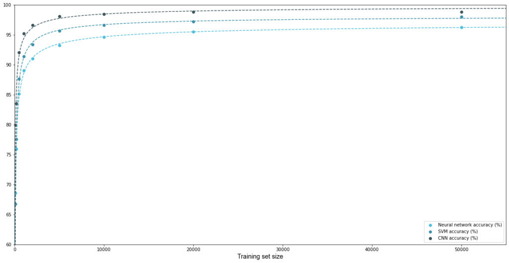
Figure 2 plots the same data points as figure 1, but this time a hyperbolic curve of best fit has been fitted for each model using the curve_fit() method in SciPy’s optimise module.
The hyperbolic curve fits the patterns we are seeing quite well, now let’s see if we can breakdown what is going on conceptually to better describe the accuracy to training dataset size trade-off.
Conceptual Breakown
At the beginning of this article, I briefly mentioned that one of the benefits of increasing the training dataset sample size is a reduction in model overfitting. We intend to create a model that predicts previously unseen circumstances based on some underlying truth in the data, rather than simply “memorising” every detail of the training dataset.
In a sense, by increasing the number of training samples we make it difficult for the model to learn from stochastic noise in the data. At the same time, we are providing more opportunity for the model to learn general underlying patterns.
To help visualise this, imagine an endless treasure hunt, where following a sequence of clues leads you closer to the position of some priceless treasure. We will assume that each clue is guaranteed to bring you closer to the treasure.
If we start our hunt with only a handful of clues, we might begin by reading each clue and walking directly to the next one. Eventually, we would have wondered to the clue that leads us to the exact location of the treasure.
However, if we had started with more clues this process could get tyring very quickly. Another way to approach the hunt would be to guess the approximate location of the treasure, based on the clues’ position rather than reading and walking to each clue.
In this case, we lose information about the exact location of each clue (and thus the final treasure) but we can be sure we are approaching the right direction.
Additionally, in this scenario the more clues we have the better our guess at “what the right direction” will be. However, the proportion of information we learn which each new clue is less and less; our guess from 5 clues might not be much different than our guess with 7 clues. Soon we will not get any closer to the treasure unless we start reading the clues.
One factor that will affect how quickly we find the direction to the treasure is our ability to infer the right direction from clues. If we were excellent at learning from underlying patterns, we might have a good guess of the direction of the treasure with only 3 clues and adding more clues might not be much help.
Similarly, the maximum accuracy we can reach is limited by how well we can guess the location of the treasure.
Here we are describing the increase of the data size (number of “clues”) solely as a method for reducing overfitting. The key here is that when offer fitting is low, our results will approach a maximum accuracy, but the amount the accuracy improves will be proportional to the number of training samples, and dependent on the model’s “learning ability”.
If the above were the case, we would assume the following to hold.
- Model complexity (a model’s “ability” to ignore noise) has some bearing on the rate at which the slowdown of accuracy improvement occurs
- A model will asymptotically approach some maximum accuracy based on its complexity
- Other methods for reducing overfitting should display a similar accuracy to training dataset size trade-off
Power to the Curve
Using the thought pattern described above, we can form a more robust estimation for our curve of best fit, the power law:
![\[Accuracy=A_{max}+c_1x^{c_2}\]](https://brentonblogs.com/wp-content/ql-cache/quicklatex.com-0e48cec37b71f7d251bcf0ae48a7c6a8_l3.png "Rendered by QuickLaTeX.com")
Where:
- x is the number of training samples
- Amax is the maximum accuracy possible (as a function of model architecture and hyperparameters)
- c1, c2 are constants that define the exact shape (slope) of the curve, also dependent on the model. Note that c2 will always be a negative real number.
Defining a curve in this way addresses the points made in our heuristic explanation above, namely the dependence of model complexity on the curve’s shape and an asymptotic approach to maximum accuracy.
Fitting a curve of this form to the accuracy data indeed provides a very good approximation. It should be no surprise, as this curve is a generalisation of our initial guess (reciprocal).
We can validate our conceptual understanding by plotting model accuracy while altering a different method for reducing overfitting. Figure 3 shows the effect of altering an L2 regularisation has on the accuracy of our shallow ANN.

Although there is some variation in the data, plotting the same power-law curve sufficiently models the effect. This suggests that reducing overfitting is indeed playing a key role in the accuracy to training dataset size trade-off.
Conclusion
There are two main insights from this investigation:
- A mathematical relationship describes how accuracy grows as training dataset size increases
- Although not the only factor, the reduction of overfitting can describe the accuracy vs training dataset size curve.
One last thing to note is that more data will almost always increase the accuracy of a model. However, that does not necessarily mean that spending resources to increase the training dataset size is the best way to affect the model’s predictive performance.